Creating a Basic Excel Export Template
New users implementing LIMS to automate their former paper-based records management often want a report equivalent to their original sample logbook. While a user-defined report (UDR) in LIMS is one solution, an Excel template offers better control of the report’s layout and appearance. We will create a simple Excel sample log report to produce a record of samples logged daily, weekly, or for any other timeframe. The sample log report can list any sample characteristics such as sample ID, batch number, customer, project, collected date, etc. The report will not list any analyses or analytical results, as that will be the topic of a future article.
Often, the easiest way to create a new template is to copy and modify an existing template. We encourage you to explore the example templates in folder C:\LIMS\Examples. However, our goal in this series of Insights articles is to learn more about a template’s macros so we will build our report from scratch.
As we learned in the previous article, every export template used with LIMS must have a LIMSData worksheet with macros BeforeTransferFromLIMS and AfterTransferFromLIMS. Since the example LIMS Export Template in folder C:\[1]LIMS\Examples\Excel Export Templates, has only a LIMSData sheet with empty versions of the two required macros, we can use it as the basis for our template. Begin by making a copy of example file LIMS Export Template.xlt then rename the file Sample Log.xlt. Note that newer versions of Excel support additional file types and extensions. However, for compatability you should continue to save all your LIMS templates in Excel 97-2003 format with an XLT extension.
Open the Sample Log template, add a new worksheet named Report before the LIMSData sheet, then close and save the template. Remember, to open any Excel template file (XLT extension) for editing either right[1]click the file in Windows Explorer and choose Open from the popup menu or open the file within Excel. Double-clicking an Excel template in Windows Explorer does not open the template file; rather it opens a new workbook created from the template.
We will design our template for LIMS’ sample summary report. Query and preview a sample summary report containing several samples then use File | Export to MS Excel Template and select the new Sample Log template. In the resulting Excel workbook’s LIMSData worksheet, you will see all of the exported LIMS data with one row for each sample queried along with a header row of LIMS field names. Explore the data available for our report (see the example below).
Recall that LIMS runs macro BeforeTransferFromLIMS before writing the sample summary report’s data to the LIMSData sheet and macro AfterTransferFromLIMS after the data transfer. So that we may use simple Excel formulas to display sample data on our Report sheet that refer to LIMS data by field name, our AfterTransferFromLIMS will begin by creating named ranges for the data on the LIMSData sheet using the row one labels for the names. For example, with named ranges we can use cell formulas like
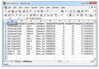
=INDEX(SampleID, 1) to display the first sample’s ID and =INDEX(Project.Name, 2)
to display the second sample’s project.
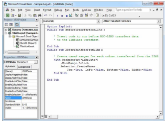
Close the workbook without saving then open the Sample Log template. Use Alt+F11 to open the Visual Basic for Applications (VBA) editor. Double-click LIMSData in the project explorer on the left then add the following lines to the AfterTransferFromLIMS macro:

Use Debug | Compile VBA Project to check for errors. If there are no errors, close the VBA editor and return to the template. The screen below shows the current state of our macro. Note that lines that begin with an apostrophe (‘) and appear in green are simply comments used to add descriptive information about the macro’s tasks.
Switch to the Report sheet in the template and add an appropriate report title and column labels. So that Excel does not attempt to use our column labels instead of our named ranges in formulas use Tools | Options and disable the “Accept labels in formulas” setting on the Calculation tab. The example below shows column labels for Sample ID, Batch, Customer, and Project. In the cell directly below the Sample ID label, add the formula =INDEX(SampleID, 1) to test. We get the #NAME? error as expected because the SampleID named range does not exist and will only be created after our macro runs.
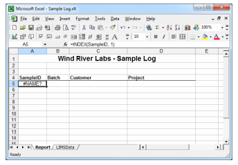
Close the template saving your changes and export the sample summary report again. Switch to the Report sheet and notice that our cell with the test formula now correctly displays the sampleID for the first sample. We could copy our sample ID cell’s formula to cells below changing the INDEX function’s row number to 2, 3, etc. but that would be tedious since we would have to copy then edit the formula for the maximum number of samples we expect to ever export from the LIMS. An alternative is to change the formula so it is relative to the cell’s current row. For example, since the sample ID formula is in cell A5, we can change it to
=INDEX(SampleID, ROW() – 4).
The ROW function returns the row number of the cell. When this formula is in cell A5 it is equivalent to
=INDEX(SampleID, 1) and =INDEX(SampleID, 2)
in cell A6. This formula is an improvement over our first attempt and it allows us to copy the formula to any number of rows below without editing. However, the formula will not have the desired result if we insert new title rows above row five. A better solution is to use a named range, as described in the following paragraph.
Following our example Report sheet above, select cells A5 through Z5, use Insert | Name | Define, enter the name “OneSample” without spaces then click the [OK] button. Although our example only uses cells A5 through D5, creating our named range through column Z allows us to add additional columns later without having to remember to update the named range. If we update our formula and make it relative to the row of the OneSample named range, we can freely insert rows above and our formulas will continue to work properly. Change the formula in cell A5 to
=INDEX(SampleID, ROW() – ROW(OneSample) + 1).
Now copy cell A5 to the other row five cells and change the SampleID field name in the formula to the column’s appropriate LIMS field name (Batch, Customer.Name, Project.Name, etc.) So that we do not have to anticipate the maximum number of samples ever exported and thereby copy our formulas to that many rows on the Report sheet, we can add a few lines of code to our AfterTransferFromLIMS macro to copy the formulas for us. Use Alt+F11 again to open the VBA editor and append the following lines below the existing lines in our macro:
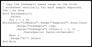
The screen below shows the updated AfterTransferFromLIMS macro. Use Debug | Compile VBA Project to check for errors. If there are no errors, close the VBA editor and return to the template.
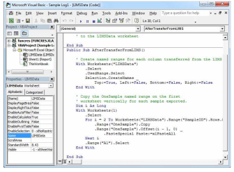
Close the template saving your changes and export the sample summary report again. Now the Report sheet is automatically visible after the macro completes and you should see one row of data for each sample exported.
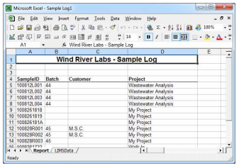
If any of the LIMS fields listed may be blank, such as batch and customer shown in the screen above, the result of our INDEX formula will display a zero. You can use Excel’s option settings to suppress all zeros on the worksheet or you can use an IF function in your formulas to suppress zeros. For example, use the formula
=IF(ISBLANK(expression), “”, expression),
where expression is the existing INDEX function.
The AfterTransferFromLIMS macro could also perform other tasks such as sorting the LIMSData sheet’s data by customer. Now that you have a basic understanding of an Excel export template’s purpose you may find it helpful to explore the macros in the LIMS example templates. Copying excerpts of code from a working template into your template is a good way to expand your Excel macro knowledge.