Creating a Basic Excel Import Template

This is the third in a series of Insights articles designed to provide a better understanding of the macros used in Excel templates. In our first two installments (see “Introduction to LIMS’ Excel VBA Macros” in LIMS Insights No. 15 and “Creating a Basic Excel Export Template” in LIMS Insights No. 16) we explored the location and names of the required macros in both LIMS export and import templates and we created a simple export template. In this article we will present the required macros for an import template.

LIMS allows users to import analysis results directly from Excel. When importing results for the same analyte across many samples, use the Results by Analyte screen; when importing results for multiple analytes for the same sample, use the Results by Sample screen. Any analyte that requires calculations to obtain a final result in the Results by Analyte screen is a good candidate for its own import template.

For our example, let’s assume our lab always uses the average of two pH meter readings to determine a pH result. We can create an import template specifically for pH, which we will use to calculate and import the average.

Begin by opening a new blank workbook in Excel, then change the name of the first worksheet from “Sheet1” to “pH” and the second from “Sheet2” to “LIMSData”.

Use File | Save, set the Save as type to “Template (*.xlt)” and the file name to “pH Worksheet”; now save the file in your Excel import templates folder (see the Workstation Configuration screen for the folder location).

Modify the layout of the pH worksheet to resemble the example below. Use cell shading to identify the cells used for data entry (white in this example). We will return to add cell formulas later.

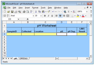
As we learned in previous Insights articles, every import template used with LIMS must have a LIMSData worksheet with macros BeforeTransferFromLIMS, AfterTransferFromLIMS, BeforeTransferToLIMS, and AfterTransferToLIMS. As their names imply, LIMS runs the macro before and after transferring the results entry screen’s data to the LIMSData sheet and before and after importing results.

When importing results by analyte, the workbook must include the anlayses’ LIMS sampleID and you will likely need to display other sample characteristics to distinguish each analysis. For this reason, an import template’s AfterTransferFromLIMS macro functions much like that of an export template. However, instead of receiving the data from a report, an import template’s LIMSData worksheet is populated with the results entry screen’s data.

Now, back in our example pH worksheet, use Tools | Macros | Visual Basic Editor to open the VBA Editor. If the Project Explorer and Properties windows are not visible on the left side of the VBA screen, use View | Project Explorer and View | Properties to display. Select Sheet2 in the project explorer and change its Name property in the Properties window to “LIMSData”. For consistency, you can also change Sheet1’s name to “pH”. Since our macros must be stored with the LIMSData worksheet, double-click the LIMSData sheet in the project explorer to open the LIMSData sheet’s VBA code window. Enter the VBA statements shown in the code window below to create the required macros.

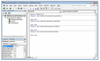
The code window above shows the four empty LIMSData worksheet macros that are required by all import templates used with LIMS. As in an export template, LIMS runs macro BeforeTransferFromLIMS before writing data to the LIMSData sheet and macro AfterTransferFromLIMS after the data transfer. However, with an import template like our pH example, the data behind the results entry screen is transferred. For each analysis displayed, one row of data is added to the LIMSData sheet. We can use the AfterTransferFromLIMS macro to redisplay sample characteristics on our pH sheet like building a report with the same macro in an export template.

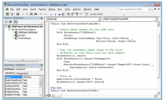
So that we can also use LIMS field names in formulas on our pH sheet to display sample data, our AfterTransferFromLIMS will begin by creating named ranges for the data on the LIMSData sheet using the row one labels for the names. Add the following lines to the AfterTransferFromLIMS macro:

‘ Create named ranges for the LIMS data With Worksheets(“LIMSData”) .Select .UsedRange.CreateNames Top:=True, Left:=False, _ Bottom:=False, Right:=False End With

The code above uses a With block, to perform multiple statements on the Worksheets(“LIMSData”) object without repeating the object name. For example, between the With and End With statements, the .Select statement is equivalent to Worksheets(“LIMSData”).Select. This code selects the LIMSData worksheet, then uses the CreateNames method on the worksheet’s used range to create names using the labels in the top row.

As in our previous Insights export template example, our macro will copy a named range of formulas on the pH sheet just once for each analysis exported; therefore we do not have to copy formulas in advance anticipating the maximum number of pH analyses we query on the Results by Analyte screen. We will add the “OneSample” named range in a moment.

Add the following lines to the AfterTransferFromLIMS macro below the lines just added:

‘ Copy the OneSample named range on the first ‘ worksheet to rows below once for each sample. Worksheets(1).Select With Worksheets(1).Range(“OneSample”) .Copy .Resize(Worksheets(“LIMSData”) _ .Range(“SampleID”).Rows.Count) _ .PasteSpecial Paste:=xlPasteAll End With

The code above simply copies the OneSample named range on the first worksheet, then pastes it to the range temporarily resized so its number of rows matches the number of samples on the LIMSData sheet. Finally, add the following lines of code to the macro to turn off Excel’s copy mode and select cell D3, the first data entry cell:

‘ Clean up Application.CutCopyMode = False Worksheets(1).Range(“D3”).Select

The screen below shows the updated AfterTransferFromLIMS macro. Use Debug | Compile VBA Project to check for errors. If there are no errors, close the VBA editor and return to the template.

Resuming our example pH worksheet above, select cells A3 through Z3, use Insert | Name | Define, enter the name “OneSample” without spaces then click the [OK] button. Although our example only uses cells A3 through F3, creating our named range through column Z allows us to add additional columns later without having to remember to update the named range. Enter the following pH sheet cell formulas:

A3: =INDEX(SampleID, ROW() – ROW(OneSample) + 1)

B3: =INDEX(CollectedDate, ROW() – ROW(OneSample) + 1)

C3: =INDEX(Location.Name, ROW() – ROW(OneSample) + 1)

F3: =IF(AND(ISNUMBER(D3),ISNUMBER(E3)), ROUND((D3+E3)/2,2), “”)

The formulas in cells A3:C3 retrieve sample characteristics by their LIMS field name from the LIMSData sheet using the named ranges created by our AfterTransferFromLIMS macro. Once you have used the template you can review the available field names on the first row of the LIMSData sheet and use any field in these and additional cell formulas. The expression “ROW() – ROW(OneSample) + 1” in each formula returns a value of 1 on row 3, 2 on row 4, etc., so that row 3 displays data for the first sample, row 4 for the second sample, etc. Note that the formulas in cells A3:C3 will result in a #NAME? error in the template, which we expect because the named ranges for the LIMS fields do not yet exist and will only be created after our macro runs.

Finally, the formula in F3 calculates the final result that will be imported into the LIMS. If cells D3 and E3 are a number, the formula calculates the average of the two rounded to two decimal places, otherwise it displays an empty string. The rounding in the formula is important because LIMS will import the cell’s actual contents, which may include more digits than displayed via the cell’s formatting. Save and close the pH Worksheet template.

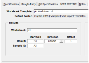
Before employing our new template for pH data entry, we must first configure the Excel interface for the analyte. The interface ties the template to the analyte and shows the LIMS where to find results to import. Open the analysis setup screen in the LIMS, switch to edit mode and select pH. Configure the Excel interface as shown below, then close the screen.

To test the template, query and display several incomplete pH analyses in the Results by Analyte screen. Use Spreadsheet | New and you should see your analyses listed in a new workbook created from the template. Enter the two pH values for each analysis to calculate the average, then return to the LIMS and use Spreadsheet | Import Results to import the averages.

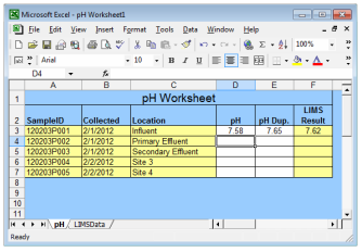
In this simple example import template, we added the four required LIMSData sheet macros and added code only to the AfterTransferFromLIMS macro. The macro created named ranges for the LIMSData sheet’s data then copied our pH sheet’s OneSample named range of formulas for the number of analyses exported, generating the worksheet above. Although we added no code to the template’s other macros, you may find them useful. For example, code could be added to the AfterTransferToLIMS macro to automatically save a copy of the workbook to a server folder whenever results are imported into the LIMS.

Copy and use this simple working example as the basis for additional templates. Explore and copy code excerpts from LIMS’ example templates to add new capabilities to your templates. Use Excel import templates to calculate and import results and eliminate duplicate data entry.